Leaf segmentation
Data labelling
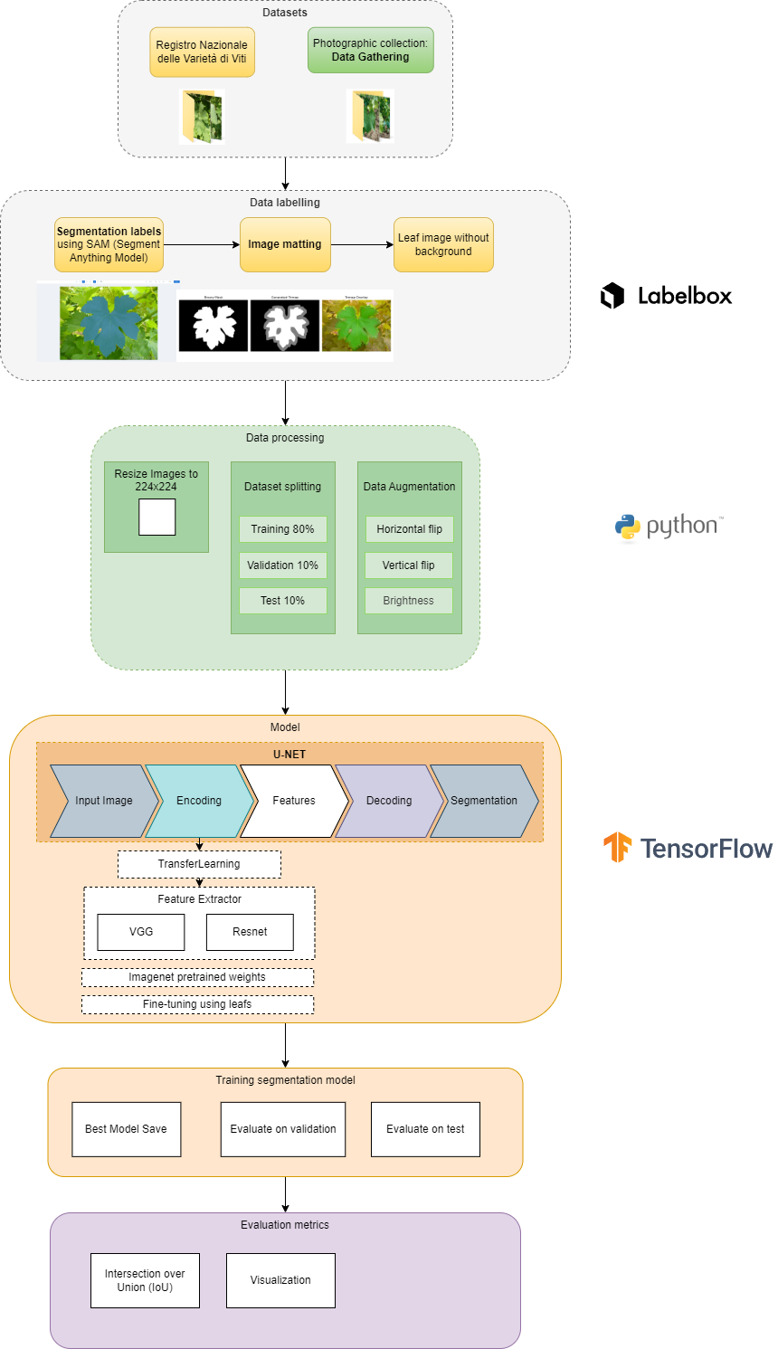
First we annotate the dataset to train deep learning models useful for better processing
Labelbox
![]()
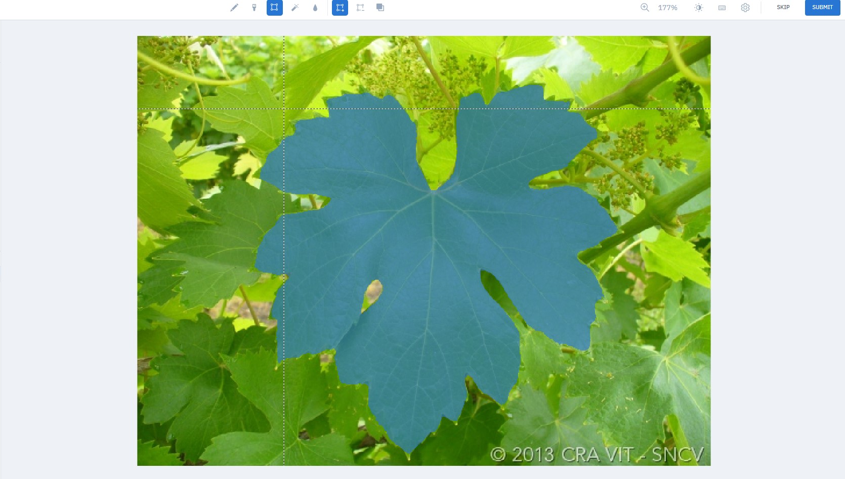
Labelbox is a very powerful platform for image annotation. It allows a simple labeling of custom image data sets. These can then be exported and used for the respective deep learning applications.
Labelbox use pre-trained models or model-assisted labeling to speed up data annotation. Like SAM model from MetaAI to segment the selected image from bounding box or point.
Workflow
1. Image annotation and review on labelbox
2. Download annotations and save them to a PNG-files
- Load Exported JSON file
- Save to a dictionary the masks urls of the original image
- Download Images using
requestswith properCookies
3. Generate Trimaps
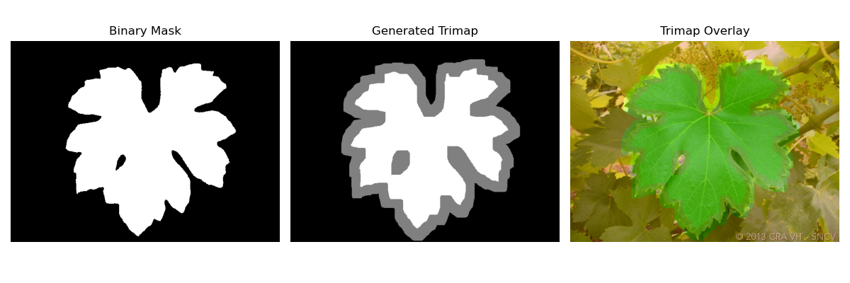
def generate_trimap(mask, kernel_size=5, fg_iter=5, bg_iter=5):
    """
    Generate a trimap from a binary mask.
    Foreground = 255, Background = 0, Unknown = 128
    """
    kernel = np.ones((kernel_size, kernel_size), np.uint8)

    # Definite foreground by erosion
    fg = cv2.erode(mask, kernel, iterations=fg_iter)

    # Definite background by dilation and inversion
    bg = cv2.dilate(mask, kernel, iterations=bg_iter)
    bg = 255 - bg  # invert to get background region as white

    trimap = np.full(mask.shape, 128, dtype=np.uint8)  # Initialize all as unknown
    trimap[bg == 255] = 0        # Background
    trimap[fg == 255] = 255      # Foreground

    return trimap
3. B Using deep learning to create the alpha matte with image matting deep algorithm
4. Modelling the image segmentation network
A neural network is used in the deep learning image segmentation to learn how to split a picture into segments. A dataset of annotated images is used to train the network, and each image is labeled with the proper segmentation. It then segment similar photos that the network has been trained for.
U-net Model
def conv_block(inputs, filters):
    x = tf.keras.layers.Conv2D(filters, 3, padding='same', activation='relu')(inputs)
    x = tf.keras.layers.Conv2D(filters, 3, padding='same', activation='relu')(x)
    return x

def encoder_block(inputs, filters):
    x = conv_block(inputs, filters)
    p = tf.keras.layers.MaxPooling2D((2, 2))(x)
    return x, p

def decoder_block(inputs, skip, filters):
    x = tf.keras.layers.Conv2DTranspose(filters, (2, 2), strides=(2, 2), padding='same')(inputs)
    x = tf.keras.layers.concatenate([x, skip])
    x = conv_block(x, filters)
    return x

def build_unet(input_shape):
    inputs = tf.keras.Input(shape=input_shape)

    # Encoder
    s1, p1 = encoder_block(inputs, 64)
    s2, p2 = encoder_block(p1, 128)
    s3, p3 = encoder_block(p2, 256)
    s4, p4 = encoder_block(p3, 512)

    # Bridge
    b1 = conv_block(p4, 1024)

    # Decoder
    d1 = decoder_block(b1, s4, 512)
    d2 = decoder_block(d1, s3, 256)
    d3 = decoder_block(d2, s2, 128)
    d4 = decoder_block(d3, s1, 64)

    outputs = tf.keras.layers.Conv2D(1, (1, 1), activation='sigmoid')(d4)

    model = tf.keras.Model(inputs, outputs)
    return model

model = build_unet((*IMAGE_SIZE, 3))
model.compile(optimizer='adam', loss='binary_crossentropy', metrics=['accuracy'])
The number of the grapevine image has been increased using different data augmentation techniques.
Evaluation
Epoch 1/30
26/26 [==============================] - 25s 888ms/step - loss: 0.7405 - accuracy: 0.7239 - val_loss: 0.6310 - val_accuracy: 0.7463
Epoch 2/30
26/26 [==============================] - 23s 855ms/step - loss: 0.5434 - accuracy: 0.7406 - val_loss: 0.4473 - val_accuracy: 0.7463
Epoch 3/30
26/26 [==============================] - 23s 856ms/step - loss: 0.4398 - accuracy: 0.7407 - val_loss: 0.4014 - val_accuracy: 0.7463
Epoch 4/30
26/26 [==============================] - 23s 859ms/step - loss: 0.4094 - accuracy: 0.8086 - val_loss: 0.3829 - val_accuracy: 0.8396
Epoch 5/30
26/26 [==============================] - 23s 858ms/step - loss: 0.3304 - accuracy: 0.8653 - val_loss: 0.1989 - val_accuracy: 0.9252
...
Epoch 29/30
26/26 [==============================] - 22s 837ms/step - loss: 0.0601 - accuracy: 0.9761 - val_loss: 0.0598 - val_accuracy: 0.9764
Epoch 30/30
26/26 [==============================] - 23s 863ms/step - loss: 0.0549 - accuracy: 0.9779 - val_loss: 0.0532 - val_accuracy: 0.9788
The network perform quite well for the amount of data used with a validation accuracy of 97% reached with 30 Epochs.
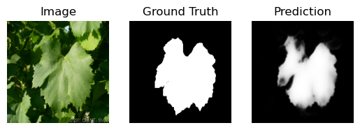
- IoU Metric also knonw as Jaccard coefficient is evaluated:
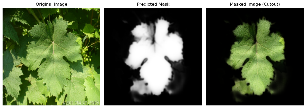
Results