Image similarity on bracelet patterns

The task of organizing pattern can be challengin, simple sorting by average color fail to capture similarities, patterns that distinguish the image and the general result is quite unpleasing.

Approach

Various method for sorting exist i gave it a try using this method:

Sorting using PCA with average color

As in this case there is no labels to train a classification algorithm we have to use unsupervised learning techniques. Recent approaches in image analysis increasingly use deep learning. Like for example This paper for clustering art paintings or artistic designs use methods such as Deep Embedded Clustering (DEC) for clustering other than commonly used, deep learning models for feature extraction.

Feature extraction

We get started by using Convolutional Neural Networks (CNNs) to extract meaningful features from the bracelet images. Some of the most popular pre-trained neural netorks are used as base model for extracting the features we will use for clustering. The choice of how to structure the neural network is given by the simplicity of our images.

Early CNN layers learn features such as edges and simple textures.
Later convolutional layers learn features such as more complex textures and patterns.
The last convolutional layers learn features such as objects or parts of objects.

Since bracelet patterns are composed of colors and geometric structures, not real world objects, we use only the early to mid-level layers from pre-trained CNNs.we don't need CNN too deep that discover objects nuances or particular details like for paintings. This preserves relevant information such as pattern, color scheme and the general low lever features of the image without many detail avoiding overfitting to irrelevant features.

Dimensionality reduction

The dataset consists by a reduced amount of images, around 10,000 bracelet pattern images are used but only 4500 are used in this example due to the fact that there are different images sizes providing too much diversity that would need more adjustment.

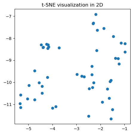
The data can be fed to the clustering model before dimensionality reduction with PCA (linear) or T-SNE(non linear) to provide better performance reducing the space of features. However in this case t-SNE was used to have a visual rappresentation of the clustering.

Pre-trained models architectures

The choise of the models is made by the most performant models of recent years.

resnet50This architecture is highly used in problems of feature extraction in computer vision
vgg19: Classic model with deep layers, effective for general-purpose visual features. The original VGG16 classifies images according to a set of 1 000 possible classes
efficientnet_b0 Efficient architecture offering a good balance between speed and accuracy.
densenet121: The name DenseNet derives from the fact that the dependency graph between the variables becomes rather dense: the last layer of the chain is densely connected to all the previous layers. they collectively contribute to the final output. Often producing compact and informative embeddings.

NOTE All those models were originally trained on datasets like ImageNet, which include natural objects, the adaptation on patters or artistic features is not trivial as the classes used for those models are quite different but the use of early-layer features helps to mitigate the difference.

from keras.layers import GlobalAveragePooling2D
from keras.applications import ResNet50, VGG19, EfficientNetB0, DenseNet121
from keras.models import Model
 
class FeatureExtractor:
    def __init__(self):
        # Dictionary mapping model names to custom extractor methods
        self.embed_dict = {
            "resnet50": self.get_resnet_feature_extractor,
            "vgg19": self.get_vgg_feature_extractor,
            "efficientnet_b0": self.get_efficientnet_feature_extractor,
            "densenet121": self.get_densenet_feature_extractor,
        }
 
    def get_resnet_feature_extractor(self):
        base_model = ResNet50(include_top=False, weights='imagenet', pooling='avg')
        return base_model
 
    def get_vgg_feature_extractor(self):
        base_model = VGG19(include_top=False, weights='imagenet')
        x = base_model.get_layer('block4_conv1').output
        x = GlobalAveragePooling2D()(x)
        model = Model(inputs=base_model.input, outputs=x)
        return model
 
    def get_efficientnet_feature_extractor(self):
        base_model = EfficientNetB0(include_top=False, weights='imagenet', pooling='avg')
        return base_model
 
    def get_densenet_feature_extractor(self):
        base_model = DenseNet121(include_top=False, weights='imagenet', pooling='avg')
        return base_model
 
    def get_feature_extractor(self, model_name):
        extractor_func = self.embed_dict.get(model_name)
        if extractor_func is None:
            raise ValueError(f"Unsupported model: {model_name}")
        return extractor_func()

Layers added From the base model no other layers are added a CNNs more close to the base model is more optimal. The feature maps are finally global average pooled to get a more compact one-dimensional vector .

Clustering

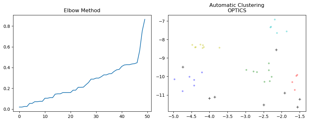
For a more diverse dataset what i found the right thing to do is use a density clustering method instead of subdividing the images into large clusters with an algorithm like DBSCAN

from sklearn.neighbors import NearestNeighbors
 
neighbors = NearestNeighbors(n_neighbors=20)
neighbors_fit = neighbors.fit(X)
distances, indices = neighbors_fit.kneighbors(X)
 
distances = np.sort(distances, axis=0)
distances = distances[:,1]
 
# Subplot Figure
plt.figure(figsize=(10, 4))
# Plot Elbow method
plt.subplot(1, 2, 1)
plt.title("Elbow Method")
plt.plot(distances)
 
'''
From KNN we can see the elbow  between 1.2 and 1.8
This is the value of Epsilon we should use
 
EPSILON -> 1.5
'''
from sklearn.cluster import DBSCAN
db = DBSCAN(eps=0.5, min_samples=4).fit(X)
 
labels = db.labels_

Elbow method To find the optimal epsilon a NN (nearest neighbour) algorithm is used to get an empirical range to the clustering through the elbow method. This approach work in the 2-dimensional space where the curve change in direction from one class to the other. However it is not interpretable as dimensionality increases especially after deep learning-based embedding.

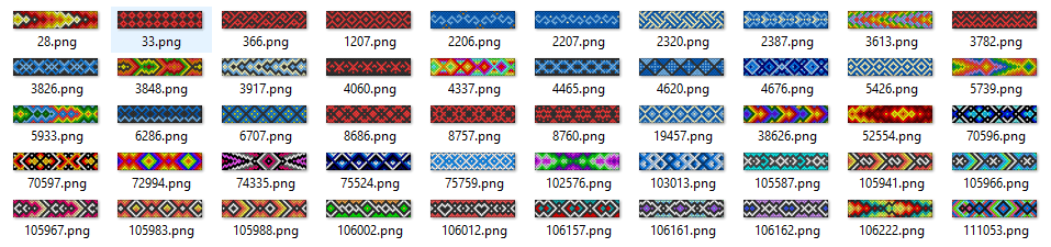
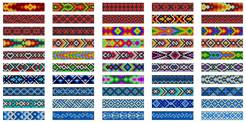
Result

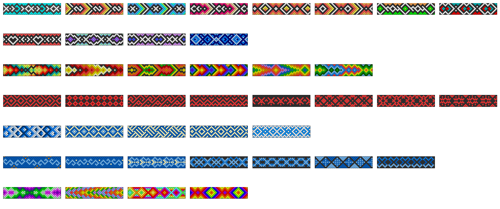
The result for a small portion of the dataset is quite pleasing.

Color groupings are preserved, meaning similar color schemes tend to appear together.
Structural patterns (e.g., stripes, diamonds, zigzags) are often grouped, proving effectiveness of the feature used.

References

[1] (A Deep Learning Approach to Clustering Visual Arts)(https://link.springer.com/article/10.1007/s11263-022-01664-y)

Image Similarity